Hello, my name is KS
I Love Engineering
Excel seems to be a important tool in data analysis.
SOME EXCEL SHORTCUTS (FOR MY OWN REVISION)
Freeze Panel / Row / Column
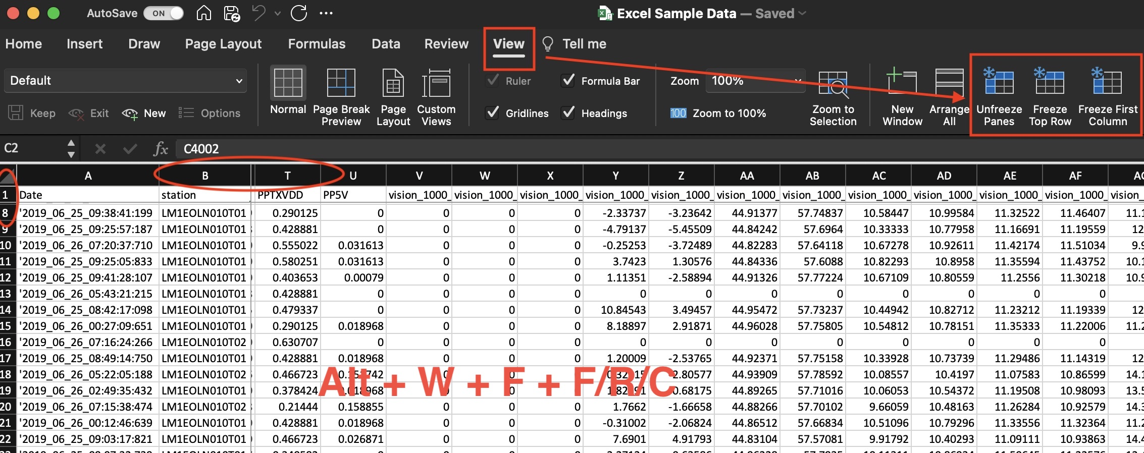
Freeze Panel Shortcut keys : Alt + W + F + F
Freeze Row Shortcut keys : Alt + W + F + R
Freeze Column Shortcut keys : Alt + W + F + C
Select Row / Column (Data Only)
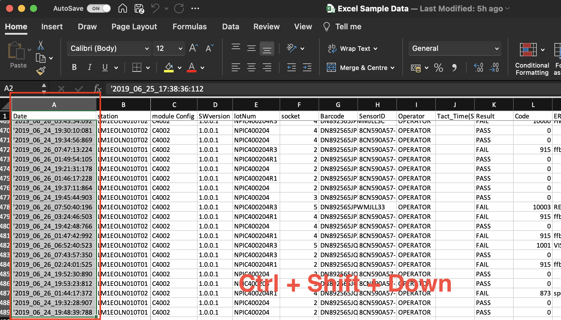
Select Row Shortcut keys : Ctrl + Shift + Down
Select Column Shortcut keys : Ctrl + Shift + Right
Select FULL Row / Column
(Include Empty Cells)
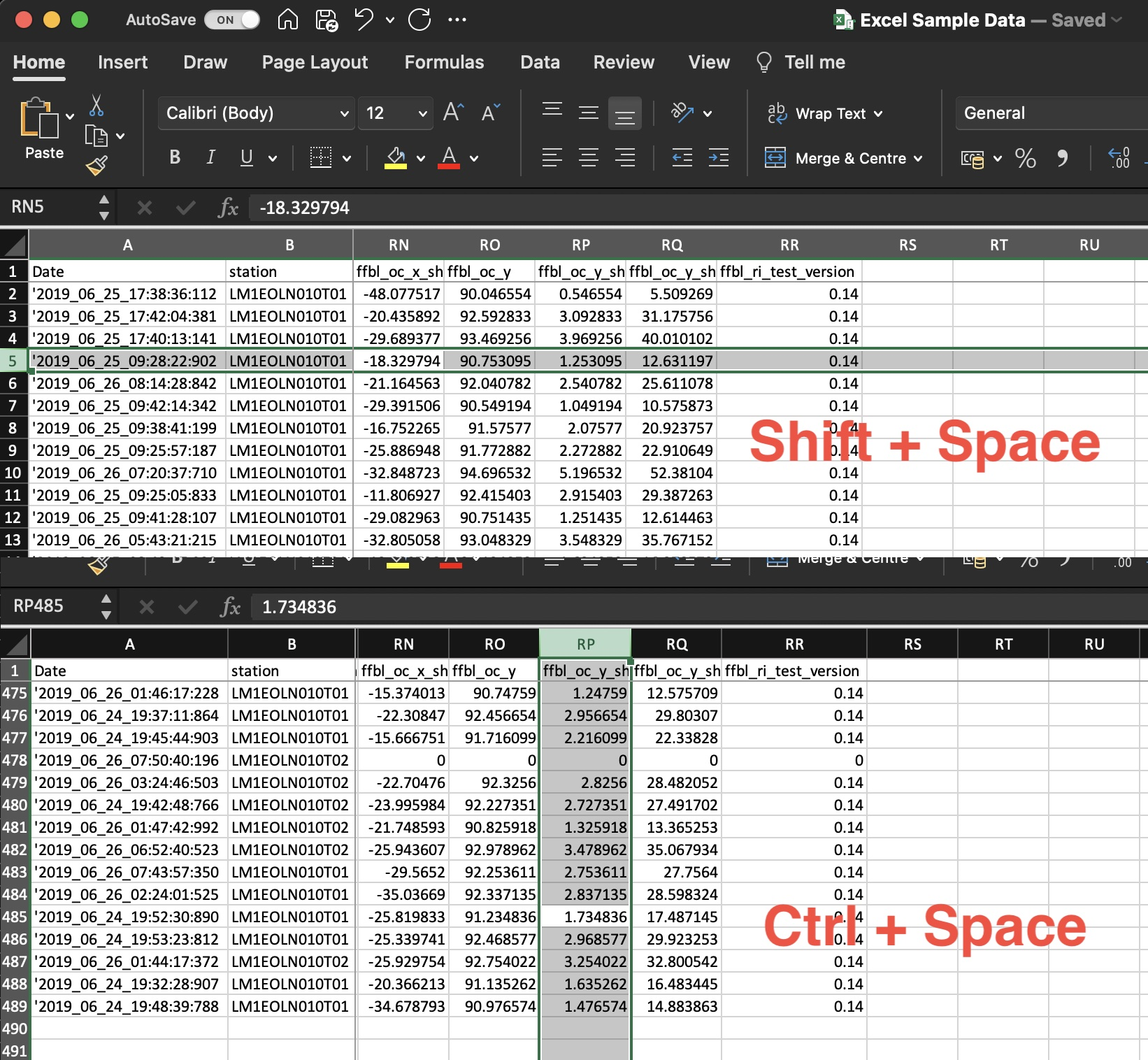
Select Row Shortcut keys : Shift + Space
Select Column Shortcut keys : Ctrl + Space
Copy Paste &
Paste Special
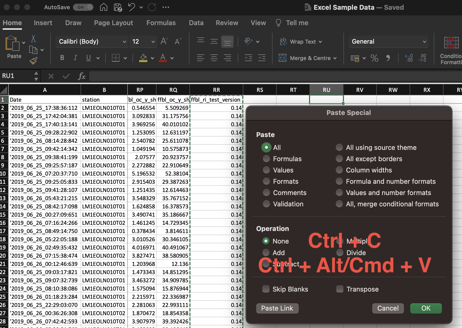
Copy Shortcut keys : Ctrl/Cmd + C
Paste Shortcut keys : Ctrl/Cmd + V
Paste Special Shortcut keys : Ctrl + Alt/Cmd + V
Add Comment / Note
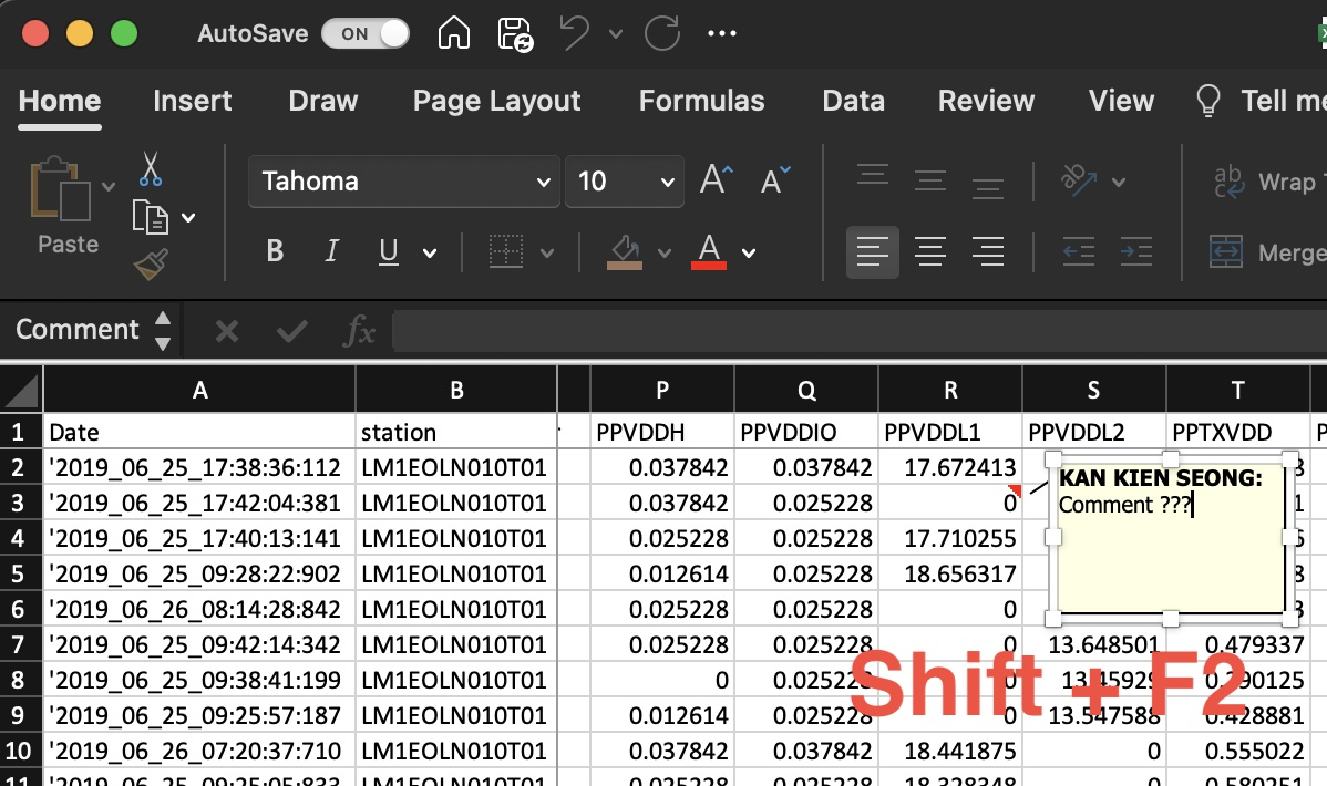
Shortcut keys : Shift + F2
Edit Format Cell
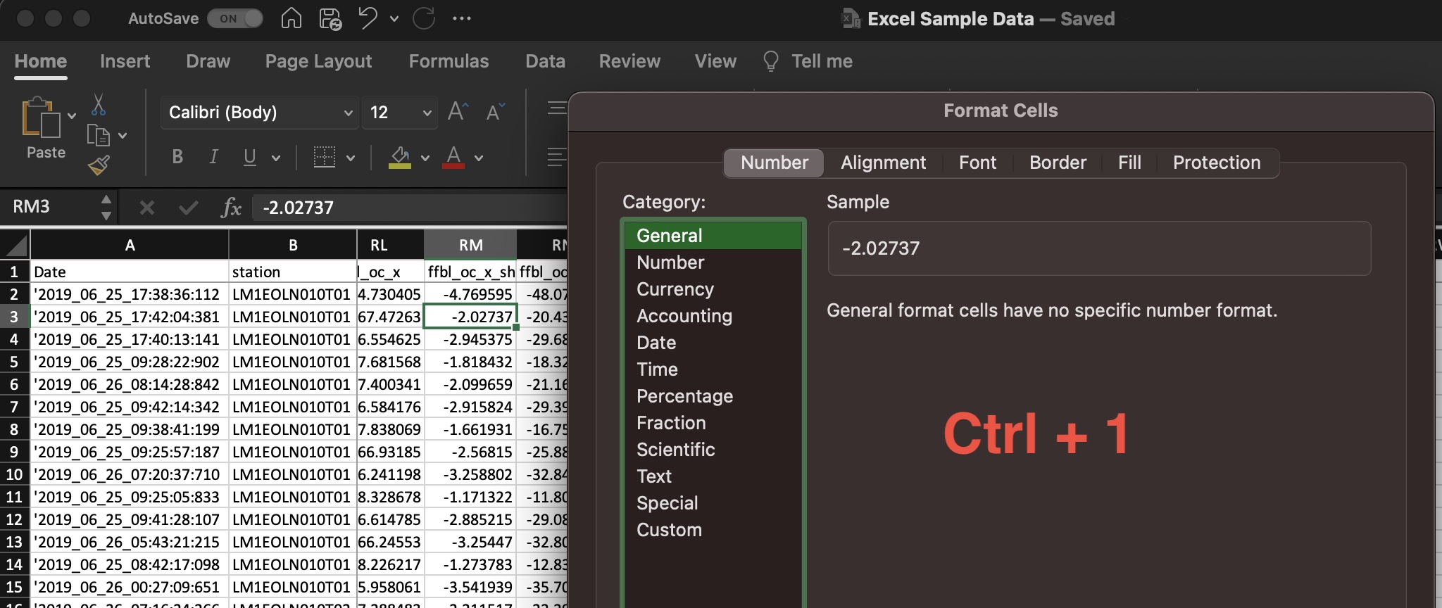
Shortcut keys : Ctrl + 1
Find & Replace Data / Formula
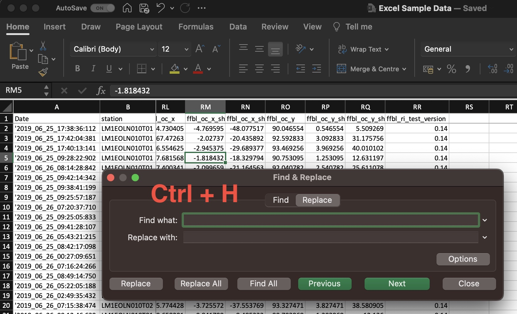
Shortcut keys : Ctrl + H
Quick filter on Specified Value
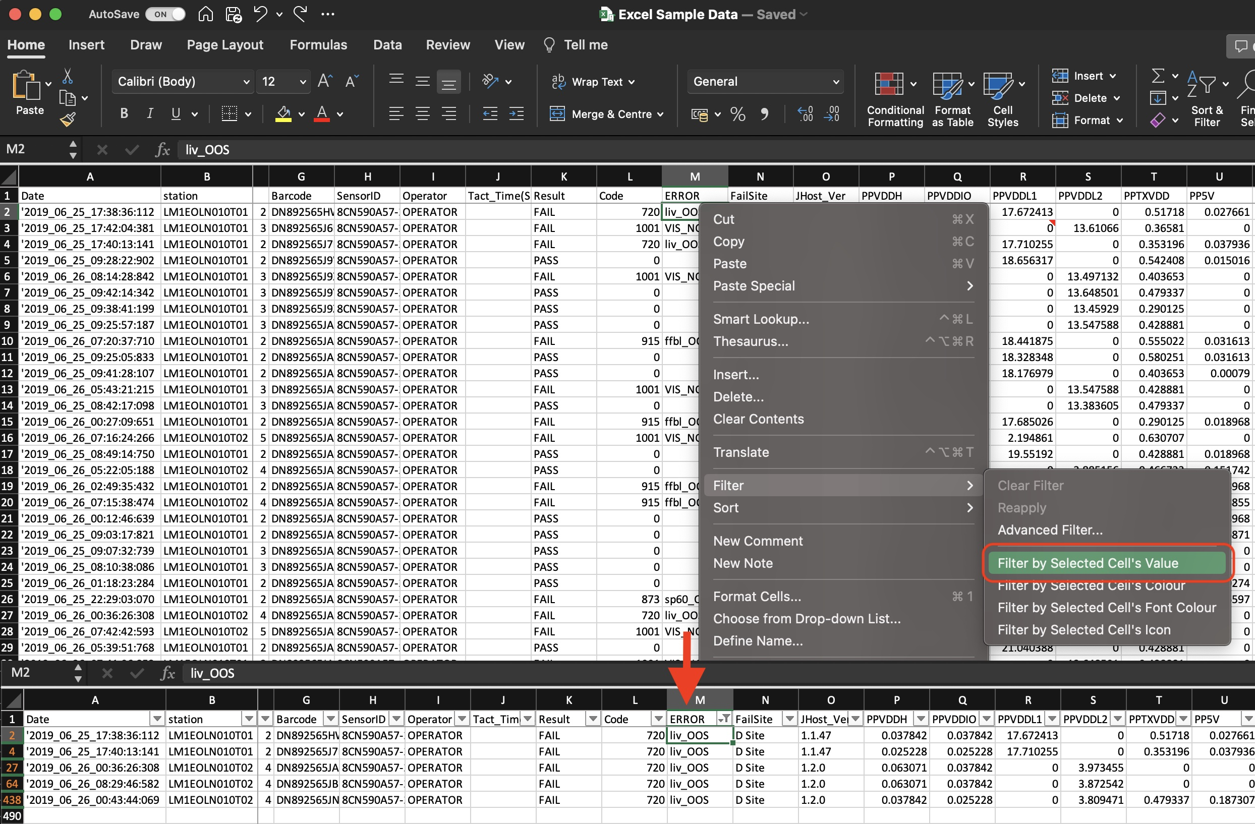
1. Right click a value in cell
2. Expand [ Filter ]
3. Select [ Filter by Selected Cell's Value ]
Convert RAW Data to Table Format
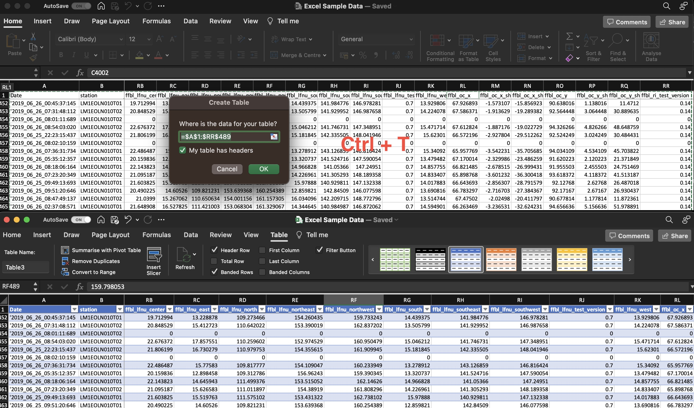
Shortcut keys : Ctrl + T
Add Slicer (Filter in Table)
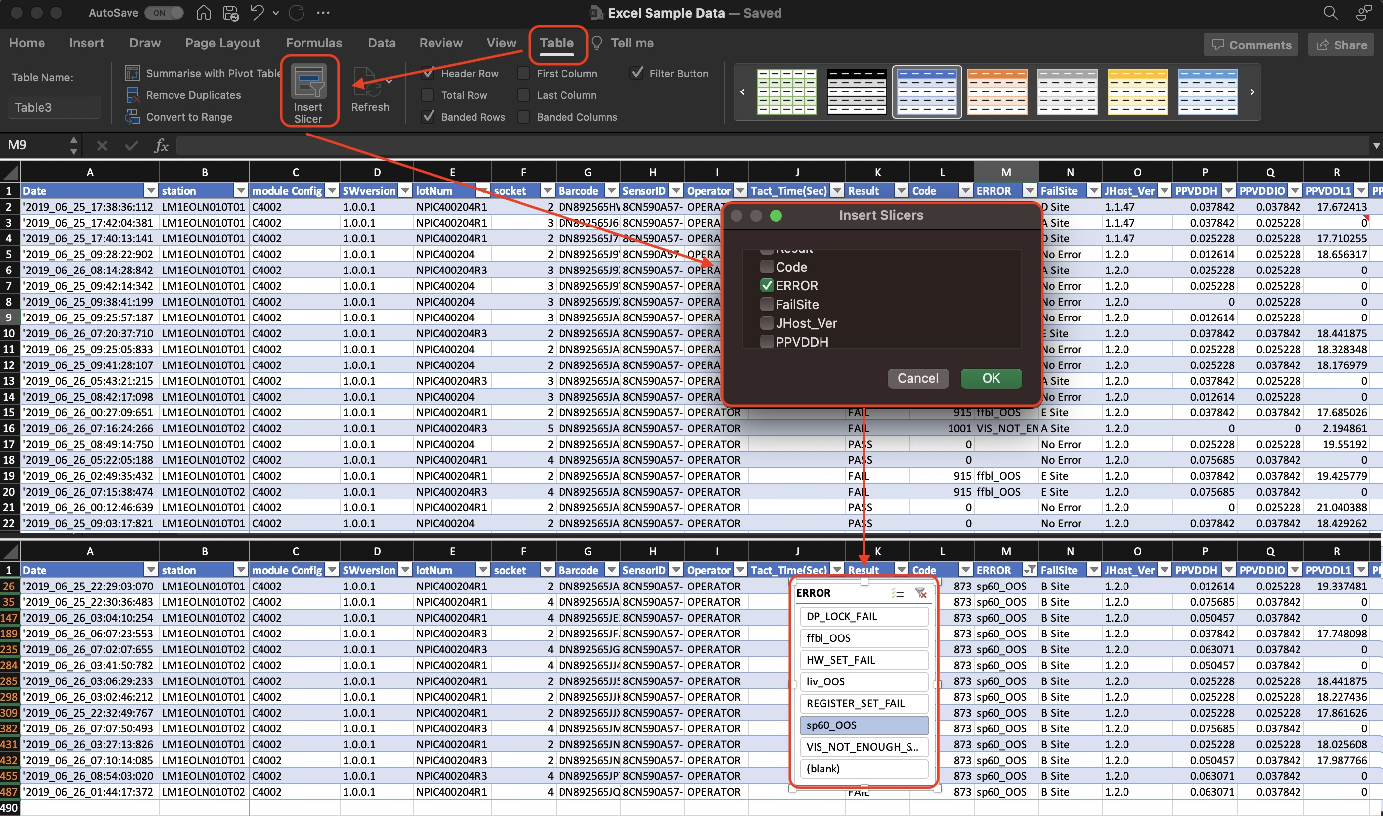
1. Select [ Table ] tab
2. Click on [ Insert Slicer ]
3. Select header for filter
4. Slicer will list out every data option for quick filter access
1st & 2nd & 3rd High Data
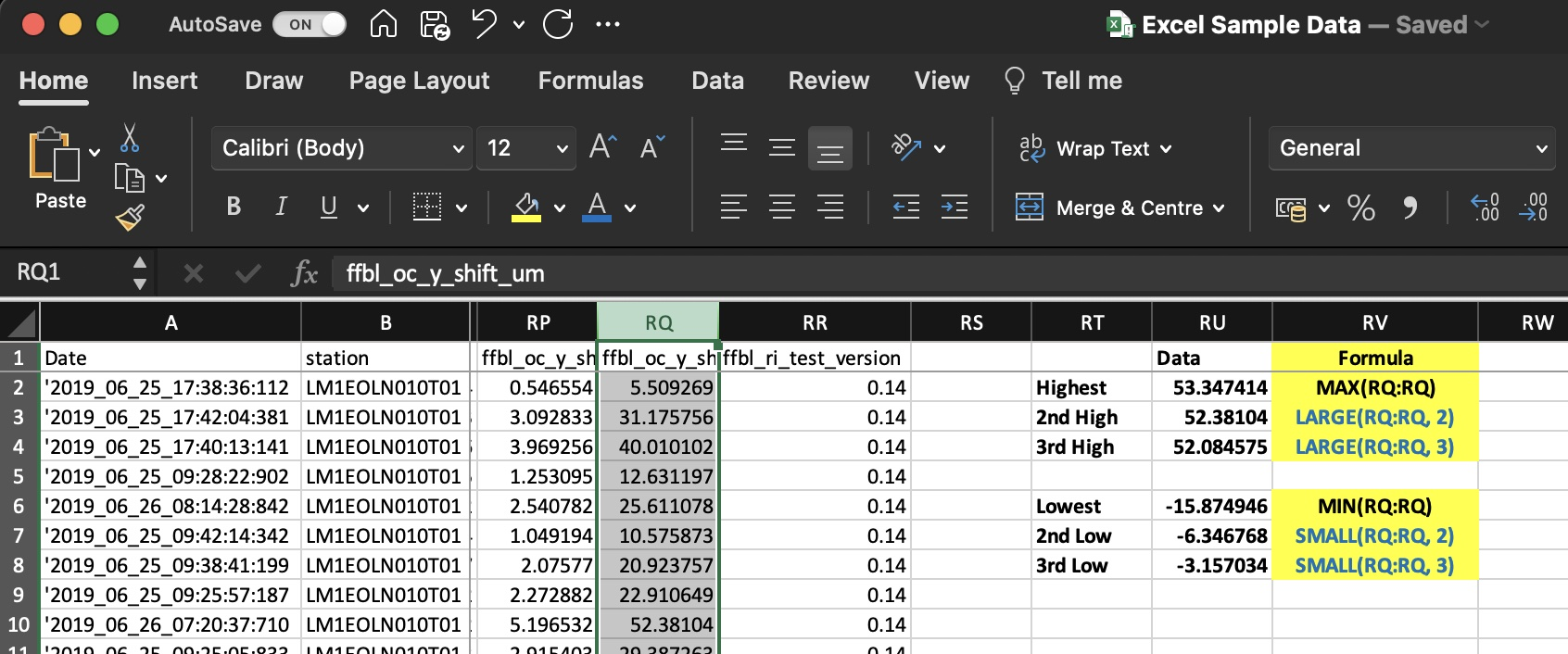
Formula to get HIGH Value :
1st : = MAX(data)
2nd : = LARGE(data, 2)
3rd : = LARGE(data, 3)
1st & 2nd & 3rd Low Data
Formula to get LOW Value :
1st : = MIN(data)
2nd : = SMALL(data, 2)
3rd : = SMALL(data, 3)
Counting with Condition
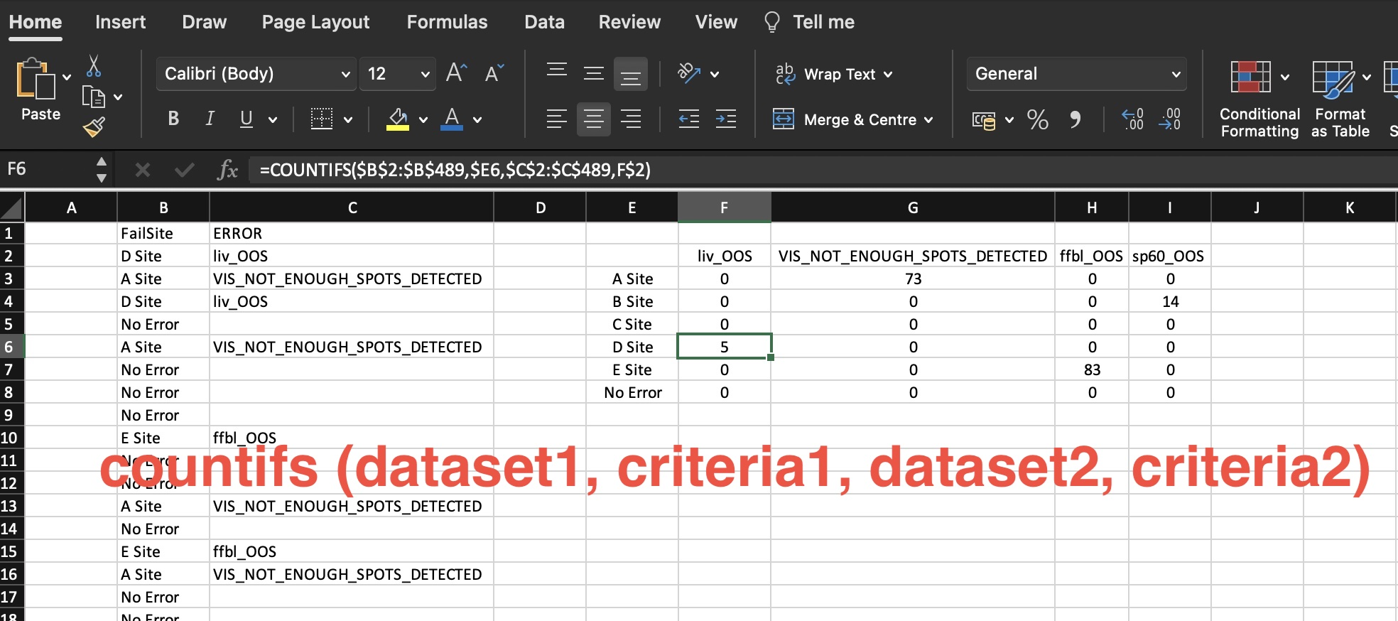
Formula couting number of data
matching selected criterias
= countifs ( Dataset1, Criteria1,
Dataset2, Criteria2 ... )
* Criteria = target data to search in Dataset
Index-Matching Condition
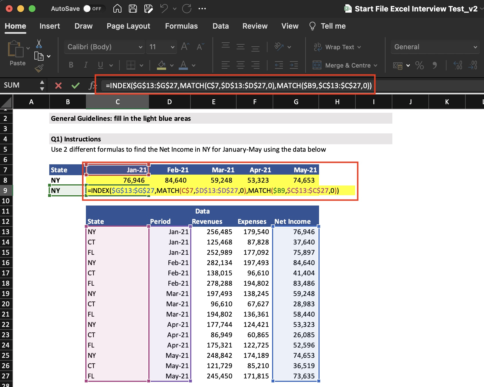
Formula pointing to a cell
when row data meeting selected criterias
= INDEX ( PoitingCellDataSet,
MATCH ( Criteria1, Dataset1 ),
MATCH ( Criteria2, Dataset2 ) ... )
* PoitingCellDataSet = Cell data will be put up if selected criterias matched
Sum up with Condition
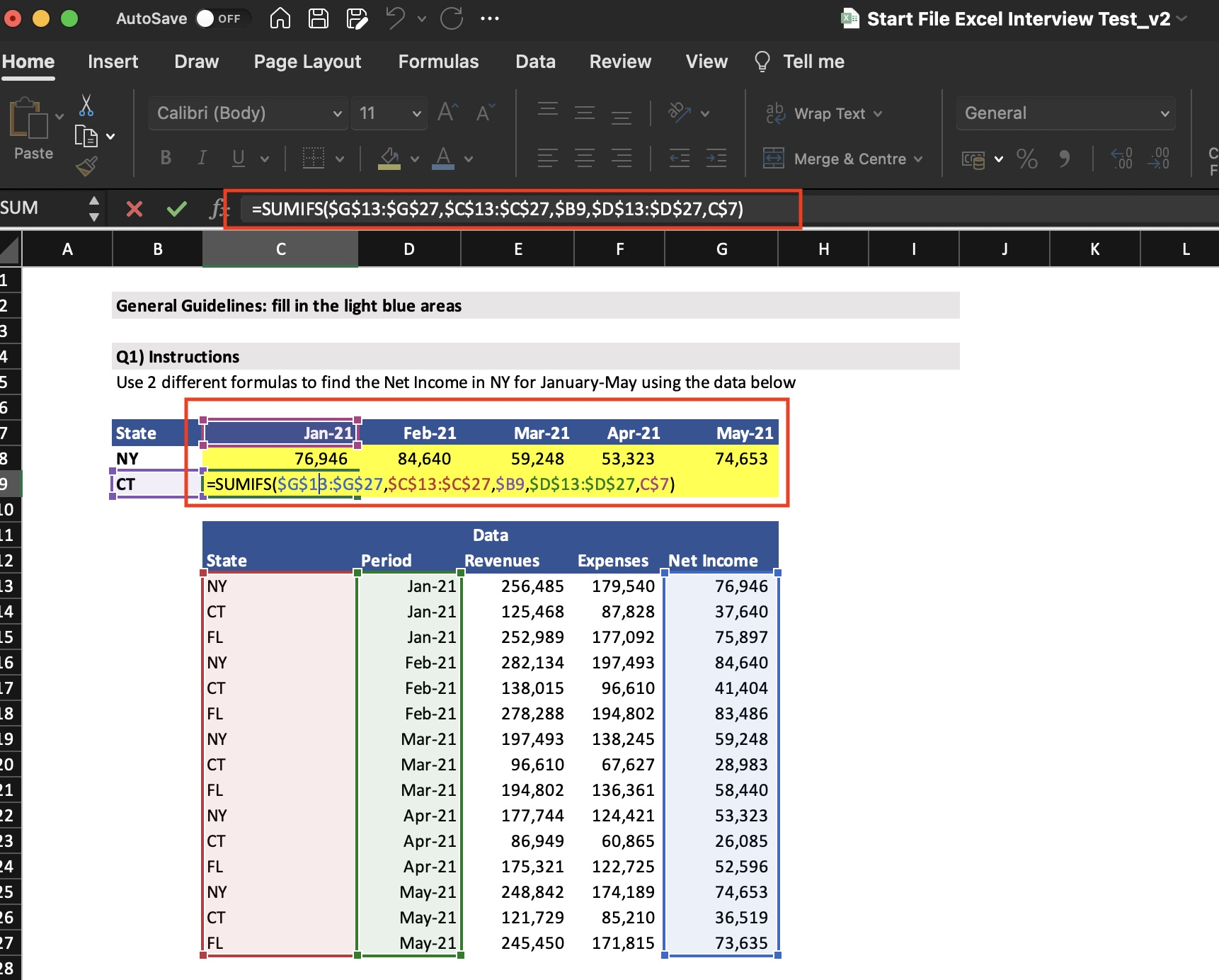
Formula sum up multiple value
that meet selected criterias
= sumifs ( SumUpValueDataSet, Dataset1, Criteria1, Dataset2, Criteria2 ... )
* SumUpValueDataSet = Value will be sum up if selected criterias matched
ComboBox
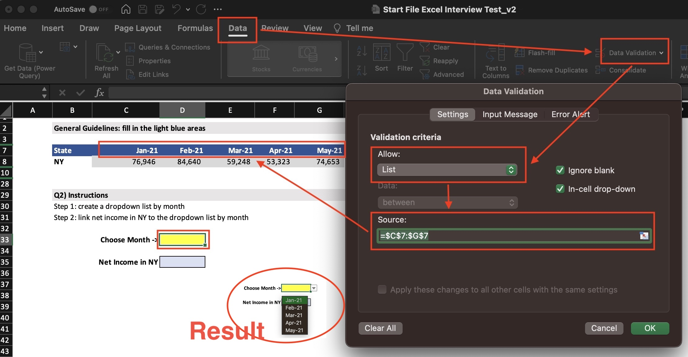
1. Select a cell to add ComboBox
2. Select [ Data ] tab
3. Click on [ Data Validation ]
4. Under Setting-ValidationCriteria-Allow, select [ List ]
5. Under Source, browse to ComboBox candidates
ComboBox
1. Select a cell to add ComboBox
2. Select [ Data ] tab
3. Click on [ Data Validation ]
4. Under Setting-ValidationCriteria-Allow, select [ List ]
5. Under Source, browse to ComboBox candidates
Datalink to ComboBox
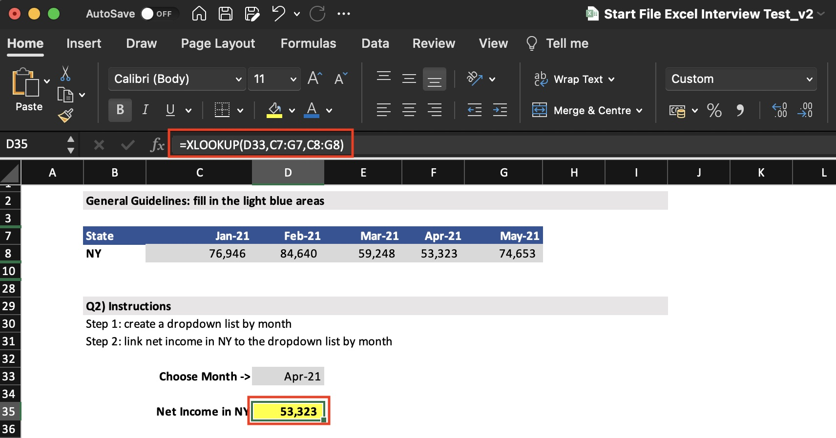
1. Dataset in a same row : = XLOOKUP ( ComboBoxData, SearchDataset, PublishDataset )
2. Dataset in a same column : = YLOOKUP ( ComboBoxData, SearchDataset, PublishDataset )
* Excel find the index where combobox data matched with search dataset item. Then retrieve same index item from publish dataset
EXCEL PIVOT TABLE
Create Pivot Table

1. Select all data on sheet
2. Select [ Insert ] tab
3. Click on [ Pivot Table ]
4. Under [ Choose where to place the Pivot Table ], select Existing Worksheet and pick an empty column/row.
5. Pivot Table space Added, click on it and you will see [ Pivot Table Fields ].
Single Category Pivot Table
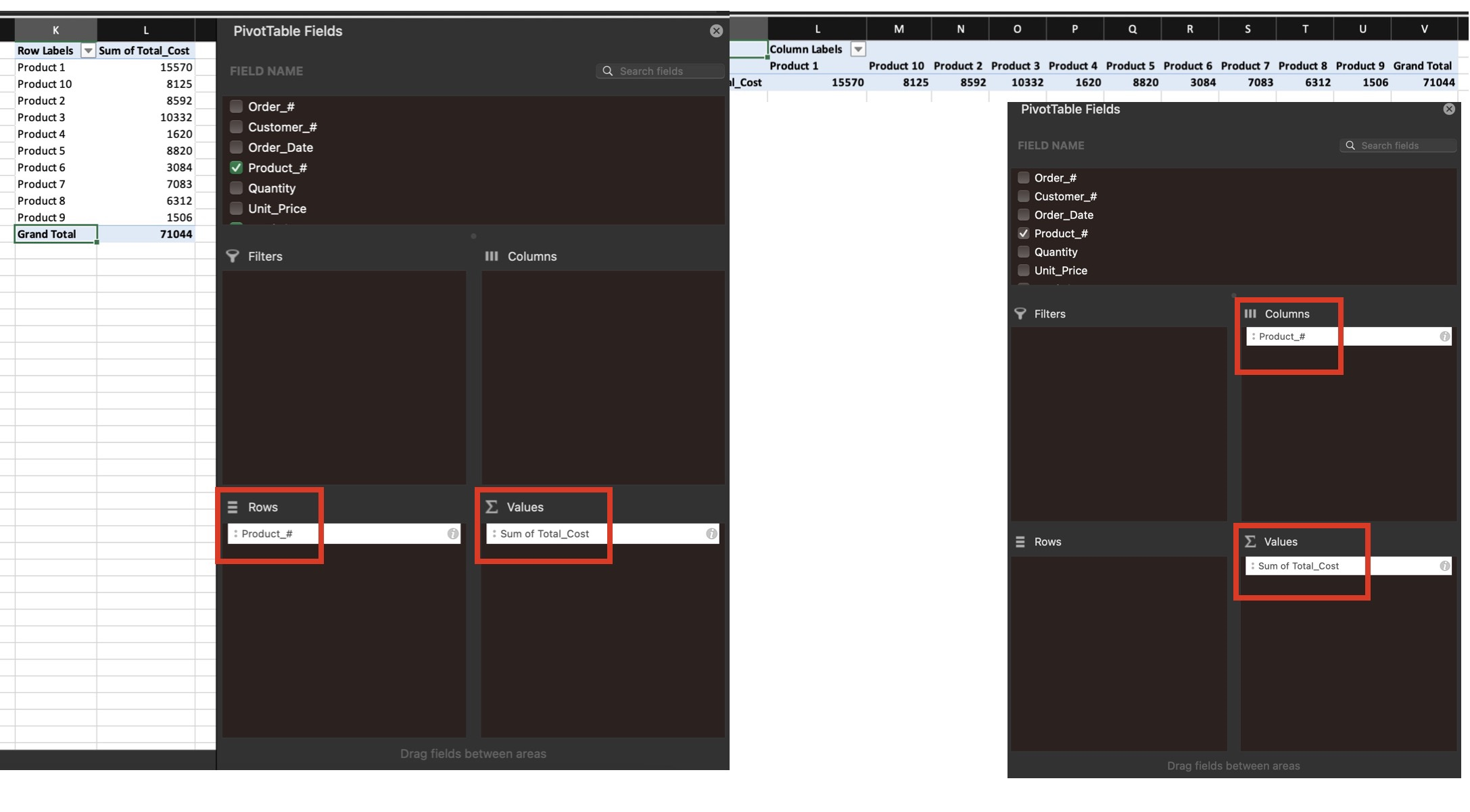
1. Drag numeric data from [Field Name] to [Values]
2. Drag category data from [Field Name] to [Rows] or [Columns]
Stacked Category Pivot Table
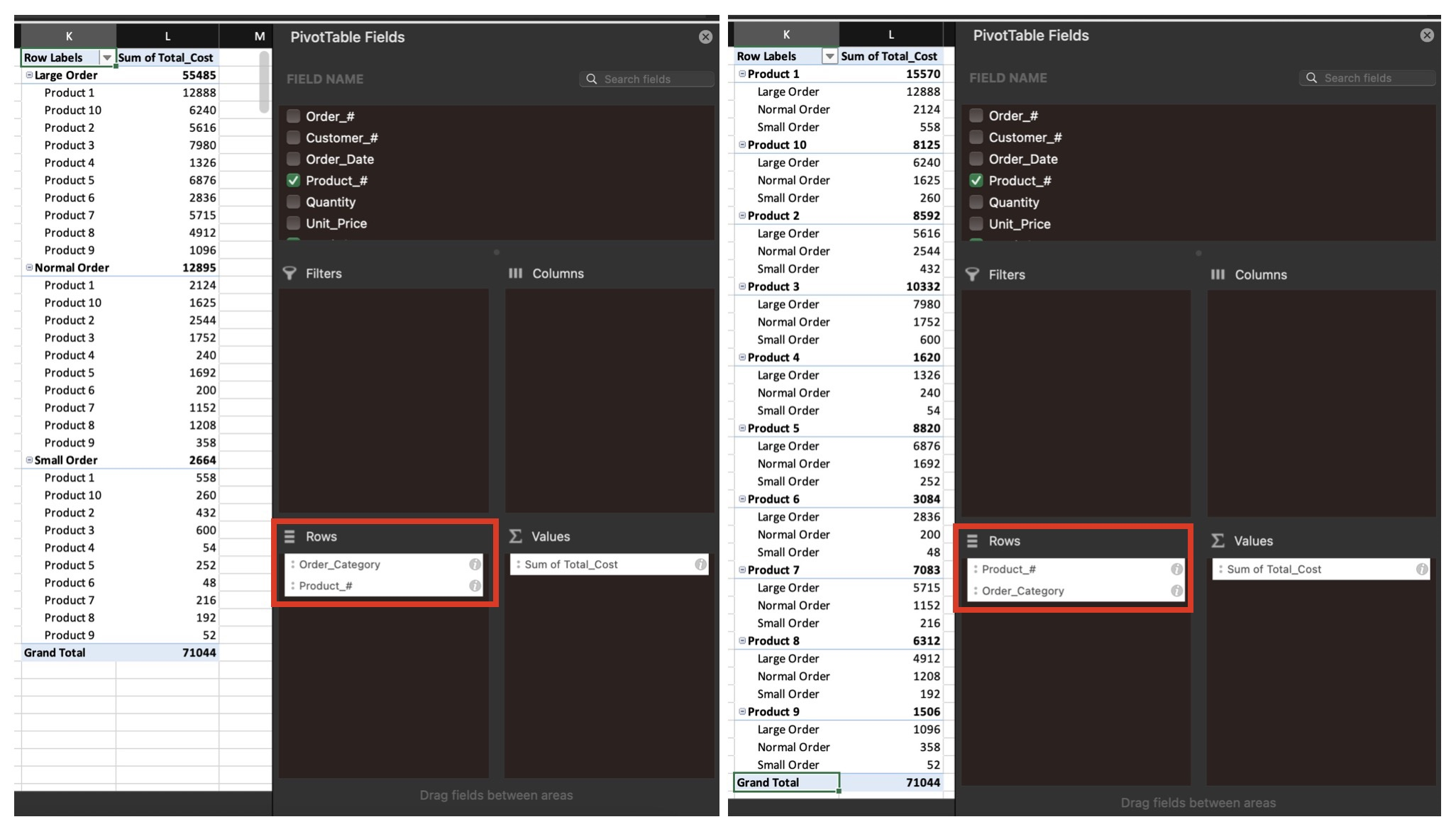
1. Drag numeric data from [Field Name] to [Values]
2. Drag 1st category data from [Field Name] to [Rows]
3. Drag 2nd category data from [Field Name] to [Rows]
** Stacked sequence do impact on output table.
Common Pivot Table
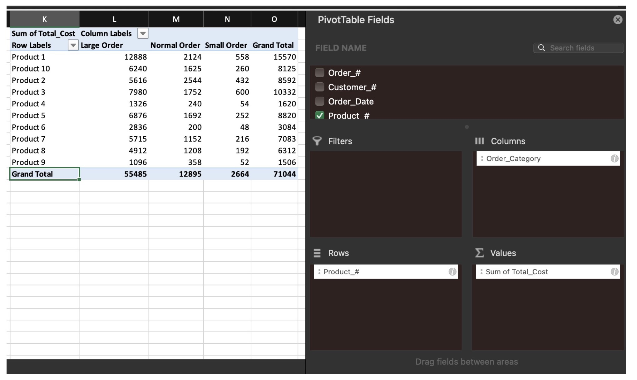
1. Drag numeric data from [Field Name] to [Values]
2. Drag 1st category data from [Field Name] to [Rows]
3. Drag 2nd category data from [Field Name] to [Columns]
Filters in Pivot Table
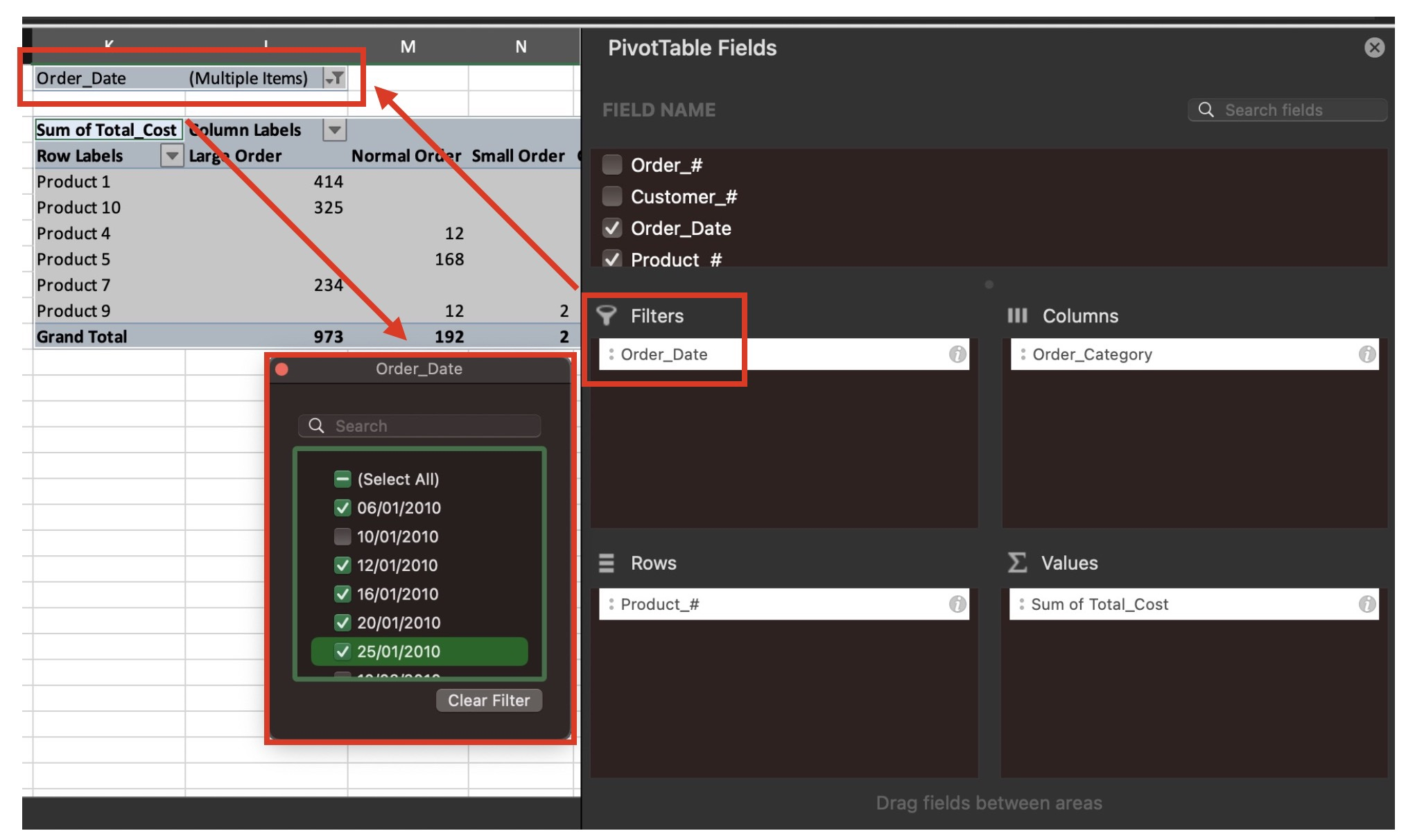
1. Drag numeric data from [Field Name] to [Values]
2. Drag 1st category data from [Field Name] to [Rows]
3. Drag 2nd category data from [Field Name] to [Columns]
4. Drag 3rd category data from [Field Name] to [Filter]
5. Select "criteria" to update the pivot table.
Chart for Pivot Table
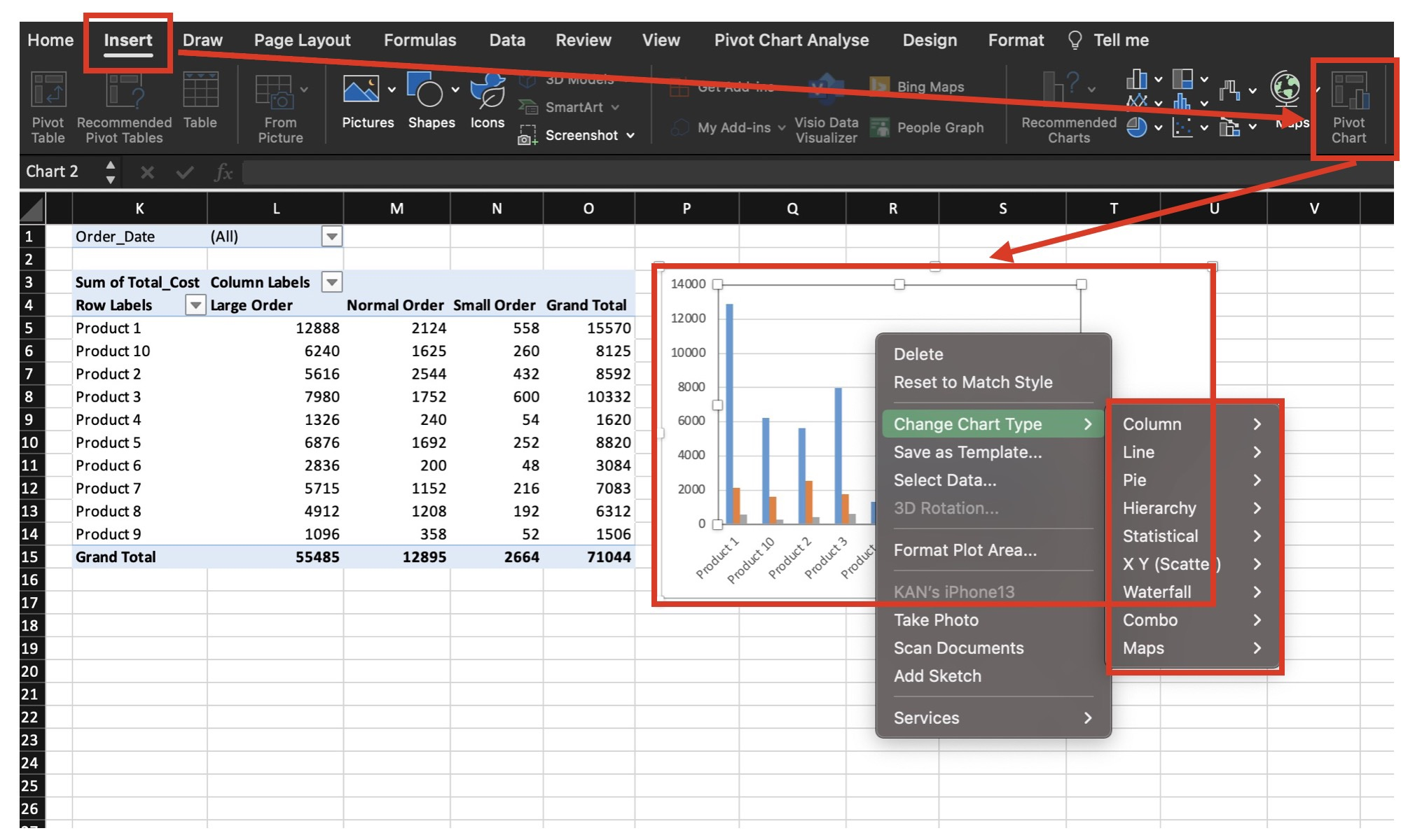
1. Select pivot table cell
2. Select [ Insert ] tab
3. Click on [ Pivot Chart ]
4. Right click on the chart, chart type & data axis can be configure here.